SECTION 4
SPATIAL DEPENDENCE
Section 4 - Spatial dependence - Looking at causes and effects in a geographical context:
- Spatial autocorrelation - what is it, how to measure it with a GIS.
- The independence assumption and what it means for modeling spatial data.
- Applying models that incorporate spatial dependence - tools and applications.
Spatial dependence
- what happens at one place depends on events in nearby places
- all things are related but nearby things are more related than distant things (Tobler's first law of geography)
- positive spatial dependence:
-
- nearby things are more alike than things are in general
- negative spatial dependence:
-
- nearby things are less alike than things are in general
- conceptual problems with negative spatial dependence
-
- e.g. the chessboard
- spatial autocorrelation measures spatial dependence
-
- an index, rather than a parameter of a process
- dependence between discrete objects, or dependence in a continuous field?
- a world without positive spatial dependence would be an impossible world
-
- impossible to map
- impossible to describe, live in
- hell is a place with no spatial dependence
- compares the squared differences in value between neighboring objects with overall variance in values
- calculates the product of values in neighboring objects
- related to Geary but not in a simple algebraic sense
Calculation of the Geary index of spatial autocorrelation
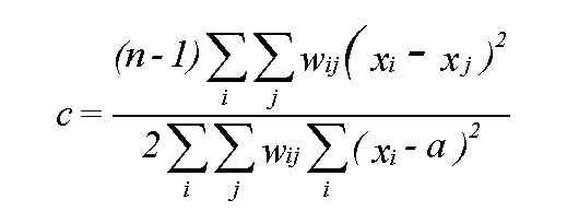
wij = 1 if i,j adjacent, else 0
c is 1 if neighbors vary as much as the sample as a whole
c < 1 if neighbors are more similar than the sample as a whole (positive dependence)
c > 1 if neighbors are less similar (negative dependence)
- i.e. neighboring values are slightly more similar than one would expect if the values were randomly allocated to the four areas
- see the discussion of variograms and Kriging
- the term geostatistics is normally associated with continuous space, spatial statistics more with discrete space
-
- Idrisi calculates autocorrelation over a raster
- code has been written to calculate autocorrelation in ARC/INFO (see NCGIA Technical Paper 91-5)
- contact Dan Griffith, Syracuse University; Luc Anselin, University of Illinois
- some of these fail to take advantage of GIS capabilities, for generating input data and displaying output
- see also Spacestat
-
- suppose there is a relationship between number of AIDS cases and number of people living in an area
- the form of this relationship will vary spatially
-
- in some areas the number of cases per capita will be higher than in others
- we could map the constant of proportionality
- spatial heterogeneity describes this geographic variation in the constants or parameters of relationships
- when it is present, the outcome of an analysis depends on the area over which the analysis is made
-
- often this area is arbitrarily determined by a map boundary or political jurisdiction
Geographically weighted regression (GWR)
fits a model such as y = a + bxbut assumes that the values of a and b will vary geographicallydetermines a and b at any point by weighting observations inversely by distance from that point
diagram
Geographical brushing:
- a technique of ESA
- a user-defined window is moved over the map
- analysis occurs only within the window
-
-
- e.g. regression analysis assumes that the observations (cases) are statistically independent
- this violates the first law of geography
- in general, analysis in space is very different from conventional statistical analysis (although this is very often carried out on spatial data)
-
- the relationship between land devoted to growing corn and rainfall in a Midwestern state like Kansas
- rainfall available at 50 weather stations
- percent of land growing corn available for 100 counties
- use a method of spatial interpolation to estimate rainfall in each county from the weather station data
- plot one variable against the other, and perhaps fit a regression equation
- how many data points are there?
-
- the more data points, the more significant the results
- 100 (the number of counties)?
- 50 (the real number of weather observations)?
- something in between?
- more data points can be invented by intensifying the sample network using spatial interpolation, but no more real data has been created by doing so
- both variables are strongly spatially autocorrelated, violating an assumption of regression
- the significance of the analysis is now uncertain
- methods of spatial regression try to overcome this problem in a systematic way
-
- see Spacestat
An example
Crime and income in Los Angelesrate of car thefts (per sq km per year)b = increase in car thefts per sq km per thousand dollars median incomemedian annual income in thousands
per census tract
5,000 observations
= -0.22R2 = percentage of variation in car thefts explained by income
= 0.26is this significant?
is it significant at the 95% level of confidence?but, but, but...we don't have a random sample of a larger populationin a population of millions of census tracts, exhibiting the same range of rates of car thefts and median incomes, but no relationship between them (b = 0, R2 = 0), could a sample of 5,000 census tracts have exhibited the same
degree of apparent relationship, or more, purely by chance?there are only 5,000 tracts in LA and we have all there is
A related issue - the MAUP
- many statistics are reported by averaging or summing over polygons - e.g. populations of counties, average elevation
- it is commonly necessary to interpolate such values to new polygons which do not coincide
-
- e.g. from census tracts with known populations to school districts
- source zones have known populations
- populations of target zones are unknown
- the best method of solving this problem is to create a continuous surface from the source data, then to integrate this surface to the new target areas
- density is constant within source zones
- density is constant within target zones
- density is constant within some third set of control zones
- density varies smoothly (Tobler's Pycnophylactic interpolation)
- e.g. Openshaw and Taylor
- 99 counties of Iowa
- two variables - % over 65, and % Republican
-
- correlation for the counties was .3466
-
6 Democrat-proposed congressional districts .6274
6 existing congressional districts .2651
6 urban/rural regional types .8624
6 functional regions .7128
- e.g. 48 regions - correlations between -.548 and +.886
- e.g. 12 regions - correlations between -.936 and +.996
- evaluate the range?
- are we asking the right question?
-
- is scale part of the question rather than a mere matter of implementation?